shapefile是GIS中非常重要的一种数据类型,在ArcGIS中被称为要素类(Feature Class),主要包括点(point)、线(polyline)和多边形(polygon)。作为一种十分常见的矢量文件格式,geopandas对shapefile提供了很好的读取和写出支持,其DataFrame结构相当于GIS数据中的一张属性表,使得可以直接操作矢量数据属性表,使得在python中操作地理数据更方便。本文给大家介绍下用Python脚本中对Shapefile文件(.shp,.shx,.dbf等格式)进行读写操作。
开发准备
由于geopandas有好几个依赖库,推荐大家使用 Miniconda或是 Anaconda来安装geopandas。
安装命令:
conda install -c conda-forge geopandas
国内镜像:
conda install -c https://mirrors.tuna.tsinghua.edu.cn/anaconda/cloud/conda-forge geopandas
使用导入:import geopandas
我这里用的是geopandas 0.7的版本,版本间差异是不太大,最新0.8版本新增了一些查询、入库方面的特性。
shapefile文件信息的读取
相比pyshp库,geopandas库的数据读取、展示、分析、拓展的效果要更好。它可以读取zip中的shapefile,还可以读取GeoJson、ArcGIS中地理数据库gdb,以及QGIS中GeoPackage 存放的矢量数据。
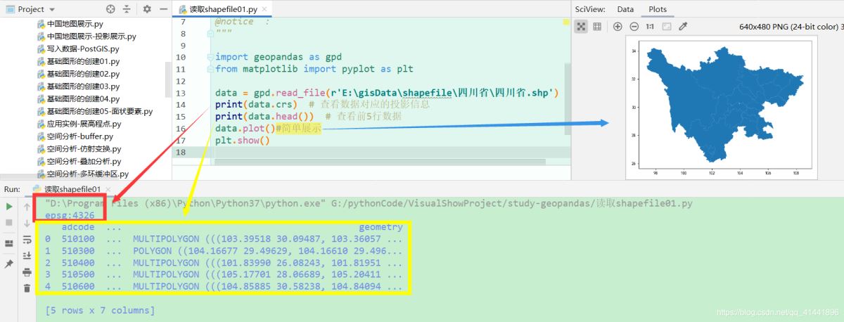
import geopandas as gpd
from matplotlib import pyplot as plt

data = gpd.read_file(r\'E:\\gisData\\行政区划数据2019\\省.shp\')#读取磁盘上的矢量文件
#data = gpd.read_file(\'shapefile/china.gdb\', layer=\'province\')#读取gdb中的矢量数据
print(data.crs)  # 查看数据对应的投影信息
print(data.head())  # 查看前5行数据
data.plot()
plt.show()#简单展示
显示效果:
shapefile文件的创建
要素类的创建效率很高,既能创建要素实体,也能写入属性信息和定义投影。下面先简单介绍下三种要素类的创建方法。
点状要素类的创建
核心代码:
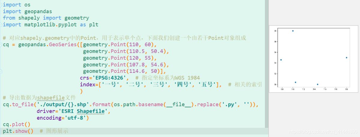
# 对应shapely.geometry中的Point,用于表示单个点,下面我们创建一个由若干Point对象组成
cq = geopandas.GeoSeries([geometry.Point(110, 60),
                          geometry.Point(110.5, 50.4),
                          geometry.Point(120, 55),
                          geometry.Point(107.8, 54.6),
                          geometry.Point(114.6, 50)],
                         crs=\'EPSG:4326\',  # 指定坐标系为WGS 1984
                         index=[\'一号\', \'二号\', \'三号\', \'四号\', \'五号\'],  # 相关的索引
                         )
# 导出数据为shapefile文件
cq.to_file(\'./output/{}.shp\'.format(os.path.basename(__file__).replace(\'.py\', \'\')),
           driver=\'ESRI Shapefile\',
           encoding=\'utf-8\')
线状要素类的创建
核心代码:
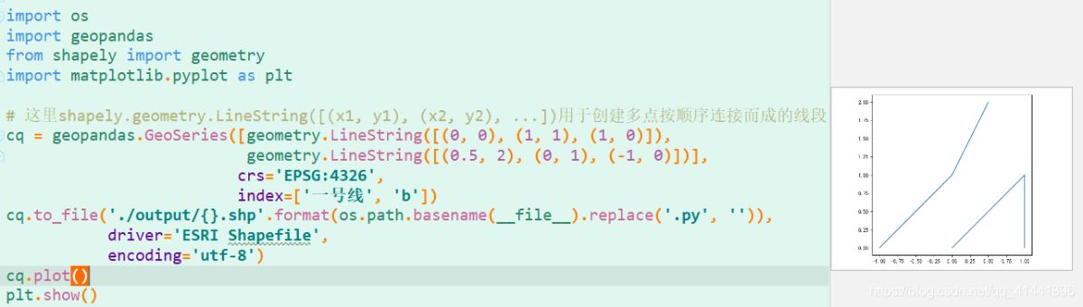
# 这里shapely.geometry.LineString([(x1, y1), (x2, y2), ...])用于创建多点按顺序连接而成的线段
cq = geopandas.GeoSeries([geometry.LineString([(0, 0), (1, 1), (1, 0)]),
                          geometry.LineString([(0.5, 2), (0, 1), (-1, 0)])],
                         crs=\'EPSG:4326\',
                         index=[\'一号线\', \'b\'])
cq.to_file(\'./output/{}.shp\'.format(os.path.basename(__file__).replace(\'.py\', \'\')),
           driver=\'ESRI Shapefile\',
           encoding=\'utf-8\')
面状要素类的创建
核心代码:
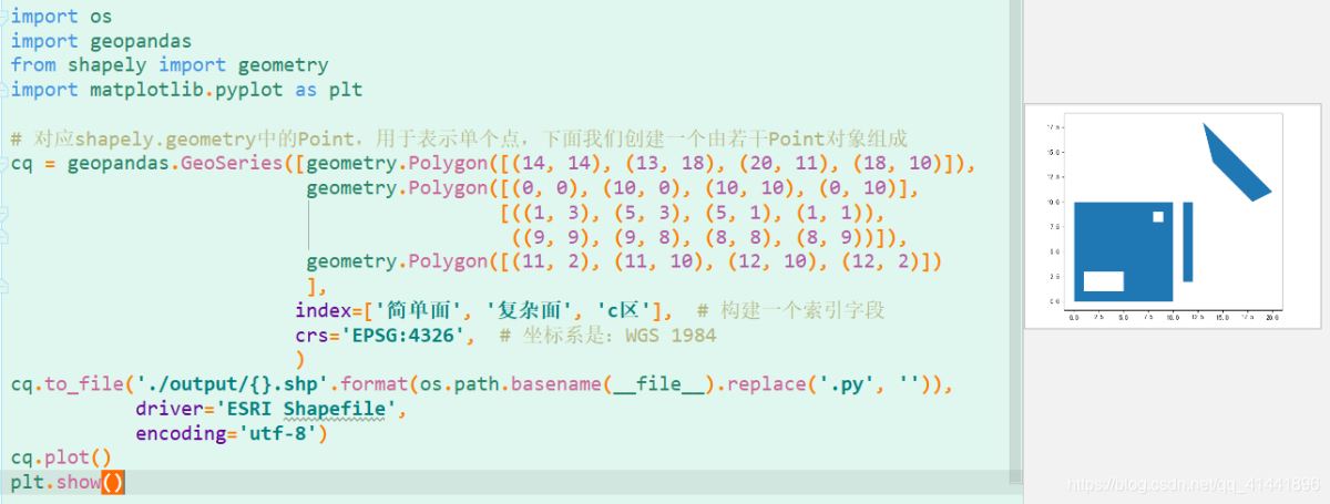
# 对应shapely.geometry中的Polygon,用于表示面,下面我们创建一个由若干Polygon对象组成
cq = geopandas.GeoSeries([geometry.Polygon([(14, 14), (13, 18), (20, 11), (18, 10)]),
                          geometry.Polygon([(0, 0), (10, 0), (10, 10), (0, 10)],
                                           [((1, 3), (5, 3), (5, 1), (1, 1)),
                                            ((9, 9), (9, 8), (8, 8), (8, 9))]),
                          geometry.Polygon([(11, 2), (11, 10), (12, 10), (12, 2)])
                          ],
                         index=[\'简单面\', \'复杂面\', \'c区\'],  # 构建一个索引字段
                         crs=\'EPSG:4326\',  # 坐标系是:WGS 1984
                         )
cq.to_file(\'./output/{}.shp\'.format(os.path.basename(__file__).replace(\'.py\', \'\')),
           driver=\'ESRI Shapefile\',
           encoding=\'utf-8\')
拓展应用实例
展高程点
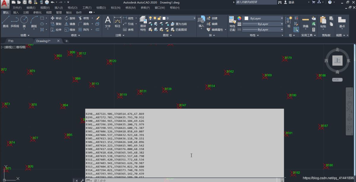
高程点文件存储格式与CASS中读取的DAT格式一致,示例:【1,ZDH ,450000.000,4100000,20002,DYG,450000.000,4100000,2000 】其中,“1”代表的是“点号”,“ZDH”代表的是“代码”,之后的分别是“东坐标、北坐标、高程值”即“Y、X、H ”或者是“X、Y、H ”
AutoCAD中展点效果
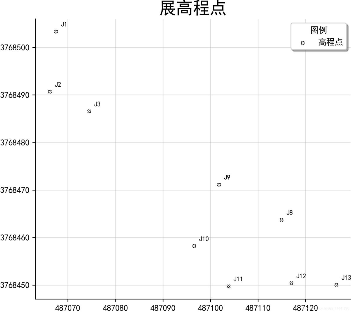
geopandas中展点效果
实现代码
# -*- coding: utf-8 -*-

import pandas as pd
import geopandas as gpd
from shapely.geometry import Point
from matplotlib import pyplot as plt
from matplotlib.ticker import FuncFormatter

# 读取数据
file_path = \'./data-use/高程数据.csv\'
rankings_colname = [\'name\', \'mark\', \'longitude\', \'latitude\', \'height\'];
df = pd.read_csv(file_path, header=None, names=rankings_colname)
# print(df.head(5))#输出前五行数据查看
xy = [Point(xy) for xy in zip(df[\'longitude\'], df[\'latitude\'])]
pts = gpd.GeoSeries(xy)  # 创建点要素数据集
#保存为SHP文件
pts.to_file(\'./output/展高程点.shp\', driver=\'ESRI Shapefile\', encoding=\'utf-8\')
\"\"\"fig是用来设置图像大小参数,ax是行列有多少个点\"\"\"
fig, ax = plt.subplots(figsize=(8, 6))  # 返回一个包含figure和axes对象的元组
ax = pts.plot(ax=ax,
              facecolor=\'white\',
              edgecolor=\'black\',
              marker=\'X\',
              linewidth=0.5,  # 内外符号比例系数
              markersize=12,
              label=\'高程点\')
# 地图标注
new_texts = [plt.text(x_ + 1, y_ + 1, text, fontsize=8) for x_, y_, text in
             zip(df[\'longitude\'], df[\'latitude\'], df[\'name\'])]


# 设置坐标轴
def formatnum(x, pos):
    # return \'$%.1f$x$10^{4}$\' % (x / 10000)#科学计数法显示
    return int(x)  # 取整显示


formatter = FuncFormatter(formatnum)
ax.yaxis.set_major_formatter(formatter)

# 美观起见隐藏顶部与右侧边框线
ax.spines[\'right\'].set_visible(False)
ax.spines[\'top\'].set_visible(False)
plt.grid(True, alpha=0.4)  # 显示网格,透明度为50%
ax.legend(title=\"图例\", loc=\'lower right\', ncol=1, shadow=True) # 添加图例
plt.title(\'展高程点\', fontdict={\'weight\': \'normal\', \'size\': 20}) # 设置图名&改变图标题字体
# 保存图片
plt.savefig(\'images/展高程点.png\', dpi=300, bbox_inches=\'tight\', pad_inches=0)
plt.show()
点集转面
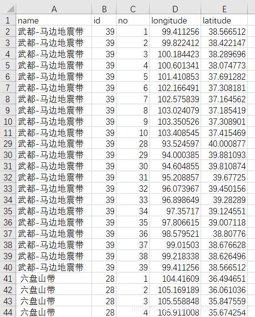
将一系列点的集合转为面状要素类,下面以甘肃省的地震带为例(字段对应:名称,面索引,点索引,经度,纬度)。
数据预览
效果预览
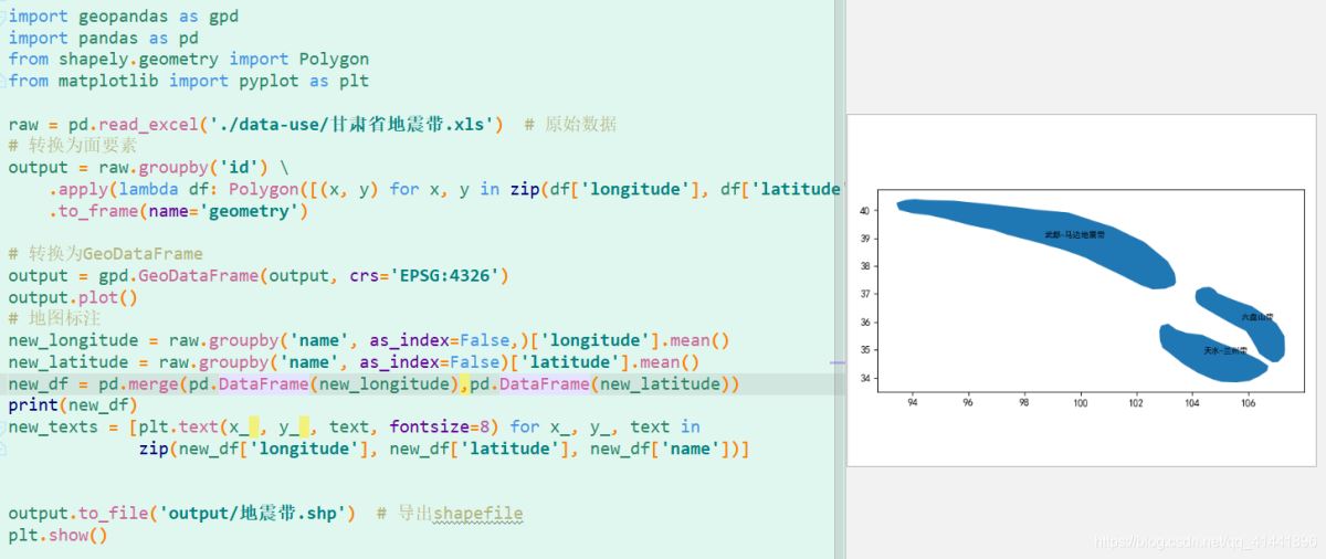

实现代码
import geopandas as gpd
import pandas as pd
from shapely.geometry import Polygon
from matplotlib import pyplot as plt

raw = pd.read_excel(\'./data-use/甘肃省地震带.xls\')  # 原始数据
# 转换为面要素
output = raw.groupby(\'id\') \\
    .apply(lambda df: Polygon([(x, y) for x, y in zip(df[\'longitude\'], df[\'latitude\'])])) \\
    .to_frame(name=\'geometry\')

# 转换为GeoDataFrame
output = gpd.GeoDataFrame(output, crs=\'EPSG:4326\')
output.plot()
# 地图标注
new_longitude = raw.groupby(\'name\', as_index=False,)[\'longitude\'].mean()
new_latitude = raw.groupby(\'name\', as_index=False)[\'latitude\'].mean()
new_df = pd.merge(pd.DataFrame(new_longitude),pd.DataFrame(new_latitude))
new_texts = [plt.text(x_ , y_ , text, fontsize=8) for x_, y_, text in
             zip(new_df[\'longitude\'], new_df[\'latitude\'], new_df[\'name\'])]
# 导出shapefile
output.to_file(\'output/地震带.shp\')
plt.show()
创建缓冲区、多环缓冲区
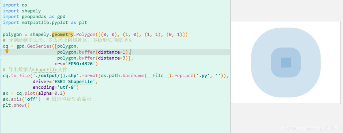
实现代码:
import os
import shapely
import geopandas as gpd
import matplotlib.pyplot as plt

polygon = shapely.geometry.Polygon([(0, 0), (1, 0), (1, 1), (0, 1)])
# 分别绘制多边形、多边形正向缓冲区,坐标系是WGS1984,单位是度
cq = gpd.GeoSeries([polygon,
                    polygon.buffer(distance=1),
                    polygon.buffer(distance=3)],
                   crs=\'EPSG:4326\')
# 导出数据为shapefile文件
cq.to_file(\'./output/{}.shp\'.format(os.path.basename(__file__).replace(\'.py\', \'\')),
           driver=\'ESRI Shapefile\',
           encoding=\'utf-8\')
ax = cq.plot(alpha=0.2)
ax.axis(\'off\')  # 取消坐标轴的显示
plt.show()
写在最后
附相关完整代码的下载,还有更多有趣的内容,感兴趣的朋友们可以自行实践。喜欢的朋友们可以点个关注,后续将持续更新,精彩无限^ – ^
链接: https://pan.baidu.com/s/1g7G8sQ17-9XIhojyQ1M7Ww
提取码: 59vz
最后给大家强烈安利一个geopandas学习博客: https://www.cnblogs.com/feffery/tag/geopandas/
以上就是python geopandas读取、创建shapefile文件的方法的详细内容,更多关于python读取shapefile文件的资料请关注自学编程网其它相关文章!